How STT Turns Vectors into Positions — Return Summaries and tanh
A visual walkthrough of JeTech STT models — encoding OHLC windows into vectors, summarizing next-day returns per similar-vector group, and mapping mean/dispersion through tanh into a position in [-1, 1].
> Status: Mechanism note. The example run did not pass the 5-year gate > (rolling 30-day average Sharpe), so the numbers below illustrate the > vector → return summary → position map. They are not a performance claim.
Question
Does an STT (statistical) model “predict price,” or does it ask: when a similar past pattern showed up, how were next-day returns distributed — and turn that into a position?
This post explains the second path with figures.
One-line summary
1. An encoder maps a recent OHLC window into a vector z. 2. Training windows’ z values are clustered into groups (default 32). 3. Each group stores next-day return mean, dispersion (std), and count. 4. Position is tanh(mean / (std + ε)) clipped to [-1, 1]; too-few samples → 0. 5. At inference: new window → z → nearest group → that group’s stored position.
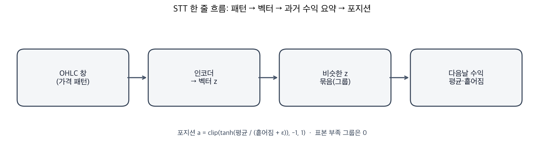
Figure 1. STT does not forecast prices directly. It looks up a past next-day return summary attached to a pattern address z.
Example run contract
| Item | Value |
|---|---|
| Run | stt_franceschi_v1_btcusdt_20260727_135008 |
| Backbone | franceschi |
| Target | BTCUSDT (solo input v1) |
| Window | 128 bars |
| Split | train 10% / test 10% / unused 80% (fixed once per seed) |
| Train windows | 170 |
| Groups | 32 |
| Min count | 5 (else position 0) |
| Label | target next-day close-to-close return only |
| 5Y gate | rolling 30d avg Sharpe ≈ 0.30 (failed; upload skipped) |
The current recommended preset sparse_v1 also uses 10%/10% train/test. The earlier first-wave design used 30%/30%.
What “probability” is actually stored
Intuitively we want “the distribution of next-day returns given this vector.” The artifact does not keep the full histogram.
Per group it stores:
mean_ret— mean next-day return of member windowsstd_ret— dispersion of those returnscount— sample sizeposition— precomputed[-1, 1]action from the summarycentroids— group centers for nearest-neighbor lookup
So “looking at a probability distribution” really means: summarize samples at train time, then look up the summary table at runtime.
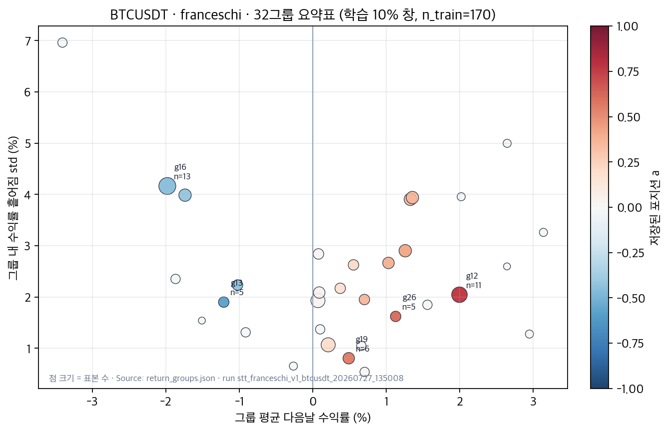
Figure 2. X = group mean next-day return (%), Y = std (%), color = stored position, point size = count. Higher mean and lower dispersion tend to push toward a stronger long position.
Largest |position| groups in this run:
| Group | Mean next-day | Std | n | Position a |
|---|---|---|---|---|
| 12 | +2.00% | 2.05% | 11 | +0.75 |
| 26 | +1.13% | 1.62% | 5 | +0.60 |
| 13 | −1.21% | 1.90% | 5 | −0.56 |
| 19 | +0.49% | 0.81% | 6 | +0.54 |
A positive mean with a large std yields a smaller score, and thus a smaller tanh position.
Visualizing the stored summary
The curves below are normal approximations drawn from stored mean/std. They are not rebuilt empirical histograms.
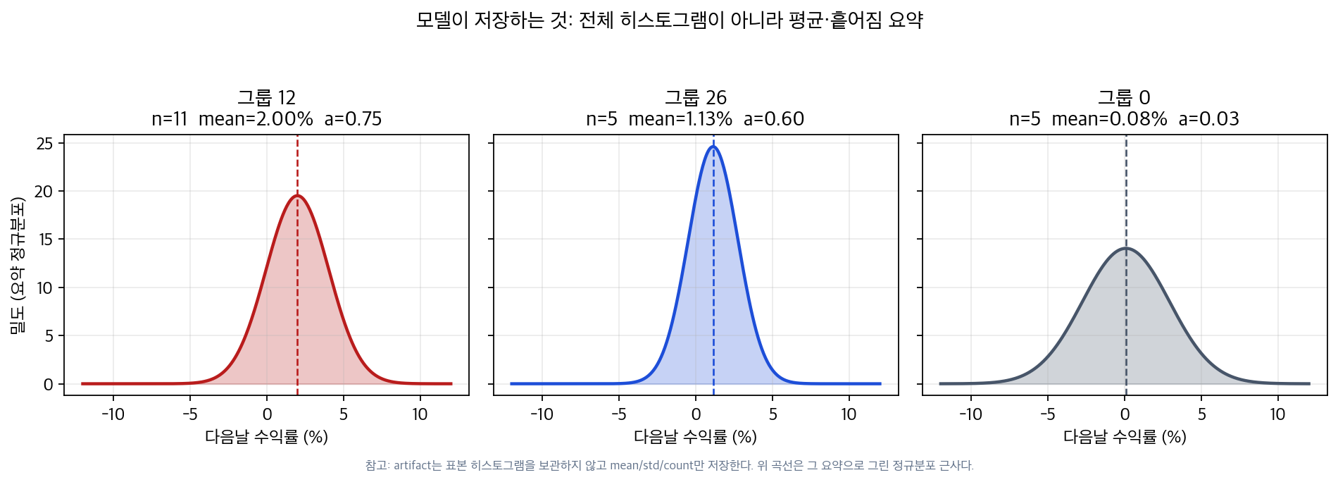
Figure 3. Group 12 sits to the right with a=+0.75. Group 26 is also positive but has only five samples. Group 0 is near zero mean and near-zero position.
The point is not that the model samples a full distribution each day. It is that groups differ in location and width, and those differences drive position size.
What tanh does
score = mean_ret / (std_ret + eps)
a = 0                  if count < min_count
a = clip(tanh(score), -1, 1)   otherwise
score asks how large the mean is relative to dispersion. tanh soft-clips that score into [-1, 1] so the model does not jump straight to full long/short. Groups with fewer than min_count (here 5) samples are forced to flat (0).
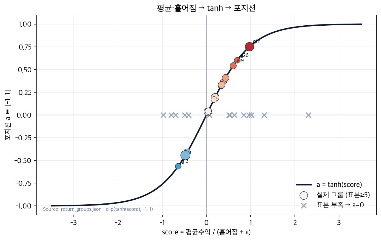
Figure 4. The curve is tanh(score). Colored points are groups with enough samples; gray crosses are forced to zero. Points on the curve mean the stored position matches the formula.
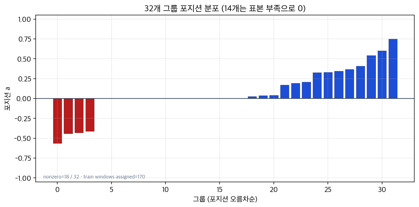
Figure 5. All 32 groups sorted by position. In this example 18 are nonzero and 14 are zero for insufficient samples. Spreading 170 train windows across 32 bins naturally leaves some bins thin.
What happens at inference
For a new decision day:
1. Build the same OHLC window. 2. Encode to z. 3. Pick the nearest stored centroid. 4. Emit that group’s stored position as the target.
Runtime does not re-estimate the return distribution. It reads the lookup table frozen at training time.
What this post does not claim
- That this example run is deployable (it failed the 5Y gate).
- That the normal approximation is the true next-day return law.
- That a 10% random train split is optimal (adjacent-window leakage and thin
samples are known risks).
- That STT beats IQL (separate contracts: STT uses real prices only; IQL trains
the policy on synthetic transitions).
Reproduce
trading/agents/runs/stt_waves/sparse_v1/stt_franceschi_v1_btcusdt_20260727_135008/

# key files
return_groups.json   # mean_ret, std_ret, count, position, centroids
stt_meta.json        # window, train/test fractions, split indices
The position formula matches fit_return_groups in trading/agents/statistical/return_table.py.
Next
- Re-encode train windows and overlay empirical histograms on the normal
approximation
- Compare position dispersion across backbones and windows (32/64/128)
- Repeat the same figures only on STT candidates that pass the 5Y gate